
You have now read and learned about the many kinds of schemas and all the different kinds of tables. Those concepts help you as an Azure data engineer to better understand the kind of data structures you could be working with. You need to know something about the data to normalize it and query to gather intelligence from. In the real world, due to the quantity of data and the speed and velocity in which things move, change happens a lot. Therefore, the tables and schemas your data analytics solution depends on will likely change too. New columns may need to be added to the tables or files, existing columns may need to be removed, and the data type you expected the value to be in may change. These are a few examples of what is referred to as schema drift. The term is used to describe the fact that there are some external dependency changes that require some attention. It is possible that you have written some code that expects an integer, but you get a string and we know that will cause an exception that stops the execution of your workflow.
You can configure your workload to manage schema drifts, as you will see later in Exercise 2.3. In summary, the platform can be configured to transform all unrecognized fields or columns into string values. If that is the case, you can code your logic to expect the same. Lastly, this concept applies primarily to static schemas. Think about why this is the case. The other scenario is a dynamic schema, which is created when you create the table that will contain the data. Therefore, you can make changes to the script that defines the schema in the dynamic context versus having to use ALTER to change a table in the context of static.
View
A database view is a table that contains data pulled from other tables. The SQL syntax to create a view contains a SELECT statement that identifies exactly which data and from which tables the view should consist of. Data targeted for a view is not persisted or cached by default; a view is considered a virtual table. This means that when you select from a view, the DBMS runs the associated query used when the view is created. Complete Exercise 2.3 to create a schema and a view using Azure Data Studio.
EXERCISE 2.3
Create a Schema and a View in Azure SQL
- Using the database that you created in Exercise 2.1, open Azure Data Studio and connect to the Azure SQL database you created in Exercise 2.1. See Figure 2.4 as a reminder of what the connection details look like.
- After successfully connecting to the database, expand the Security folder, which is below the Server endpoint URL in the Servers menu. Expand the Schemas folder and view the list of existing schemas.
- Right‐click the server endpoint URL in the Server menu, select New Query, and execute the following SQL syntax:
CREATE SCHEMA views
AUTHORIZATION dbo
4. Refresh the list of schemas to see the new schema named views. Execute the following SQL syntax from the Query window to create a view:
CREATE VIEW [views].[PowThetaClassicalMusic]AS SELECT RE.READING_DATETIME, RE.[COUNT], RE.[VALUE]
FROM [SESSION] SE, READING REWHERE SE.MODE_ID = 2 AND SE.SCENARIO_ID = 1 AND RE.FREQUENCY_ID = 1
5. Expand the Views folder to confirm the successful creation of the view. Then execute the following SQL syntax to count the total number of rows, and 10 rows from the database view the output will resemble that shown in Figure 2.18.
SELECT COUNT(*) FROM [views].[PowThetaClassicalMusic]
SELECT TOP 10 * FROM [views].[PowThetaClassicalMusic]
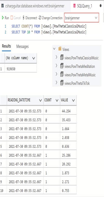
FIGURE 2.18 SQL Query from view table and new schema
You will notice in Figure 2.18 that there are a few more views and some additional data. Both the database and the queries to create the schema and view in Exercise 2.3 plus the additional views are downloadable from GitHub in the Chapter02/Ch02Ex03 folder in this repository: https://github.com/benperk/ADE. The SQL Server Authentication password for the compressed BACPAC (database backup) file is AzureDataEngineer2022 and the user ID is benperk. You can import the database by selecting Import Database on the SQL Server blade in the Azure portal.
You might be wondering why you are working with an Azure SQL database instead of a SQL pool in Azure Synapse Analytics. The reason is that you built this and the Azure Cosmos DB so that you have something to import and copy data from later, after you get through all these necessary terms and concepts. You need to know these basic things before you start building, configuring, and consuming data using those Big Data analytics tools.
In Azure Synapse Analytics there is a special kind of view called a materialized view. You create it using the following SQL syntax:
CREATE MATERIALIZED VIEW [views].[mPowThetaClassicalMusic]WITH(CLUSTERED COLUMNSTORE INDEX,DISTRIBUTION = HASH([FREQUENCY_ID]))
AS SELECT RE.READING_DATETIME, RE.[COUNT], RE.[VALUE]
FROM [SESSION] SE, READING RE
WHERE SE.MODE_ID = 2 AND SE.SCENARIO_ID = 1 AND RE.FREQUENCY_ID = 1
Notice that in this context you can set a DISTRIBUTION argument of either HASH or ROUND‐ROBIN. An advantage to creating a materialized view is that it will be persisted, unlike a default view. In general, a materialized view will improve performance of complex queries, ones that employ a JOIN and/or an aggregate. (JOIN and aggregates are discussed later.) A materialized view improves performance because the complex query was used beforehand to build the view table and populate it with data. Once that happens, instead of running the complex, high‐impact query multiple times, you run a simple query on the view to get the results quickly. To create a view using PySpark, execute the following. Note that you cannot create a persistent view on a Spark pool.
%%pyspark
data =’abfss://<uid>@<accountName>.dfs.core.windows.net/Tables/SCENARIO.csv’
df = spark.read.format(‘csv’) \
.options(header=’true’, inferSchema=’true’).load(data)
df = spark.createDataFrame(data, schema=skema)
df.registerTempTable(‘tmpSCENARIO’)
%%sql
spark.sql(‘CREATE VIEW tmpPowThetaClassicalMusic AS SELECT …’)
spark.table(‘tmpPowThetaClassicalMusic’).printSchema
spart.sql(‘SELECT * FROM tmpPowThetaClassicalMusic’).show()
The last concept we’ll examine in this context has to do with something called pruning.